Quick start

Note

Time required: ~15 min.

LocMoFit fits a geometry to single structures in SMLM data. In this tutorial, you will learn how to do this with the LocMoFit GUI in SMAP (what is SMAP?).

We will be using the nuclear pore complex (NPC) as an example. This complex appears as rings if you see them in the top view.

Task

Fitting a 2D ring model to the top-view projection of NPCs to find their positions.

Requirement

• Software: SMAP installed. Further information can be found on our GitHub site.

• Localization data: U2OS_Nup96_BG-AF647_demo_sml.mat

Main tutorial

Preparation

1. Start SMAP (how to?).

2. Load the localization data (how to?) U2OS_Nup96_BG-AF647_demo_sml.mat. This file contains segmented NPCs that you will be analyzing in the following steps.

Note

How was the segmentation done? You can check out all the pre-processing steps from fitting raw data (raw camera frames) to segmentation of NPCs in SMAP_manual_NPC.pdf.

The current window:

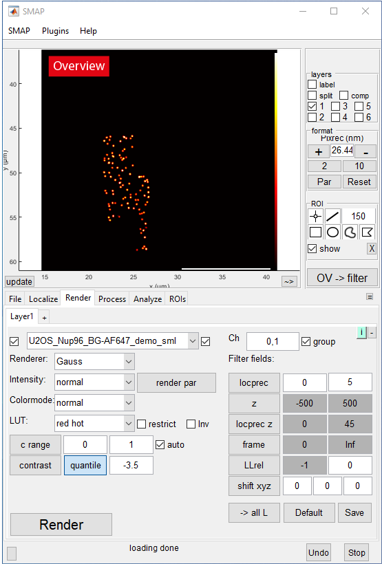
You should see the data set displayed in the Overview.

Warm-up

Before fitting, let us explore the data a bit first. We can find the list of segmented NPCs in the ROIManager:

1. Go to [ROIs] -> [Settings], click show ROI manager. This opens the ROIManager in a new window.

   Note

   ROIManager allows you to manage ROIs in different cells and files. Check section 8.2 (Manually generating a list of ROIs) in SMAP_manual_NPC.pdf for more information.

   

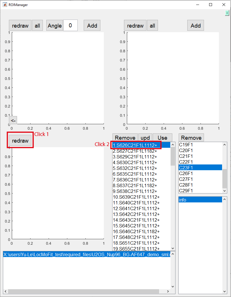
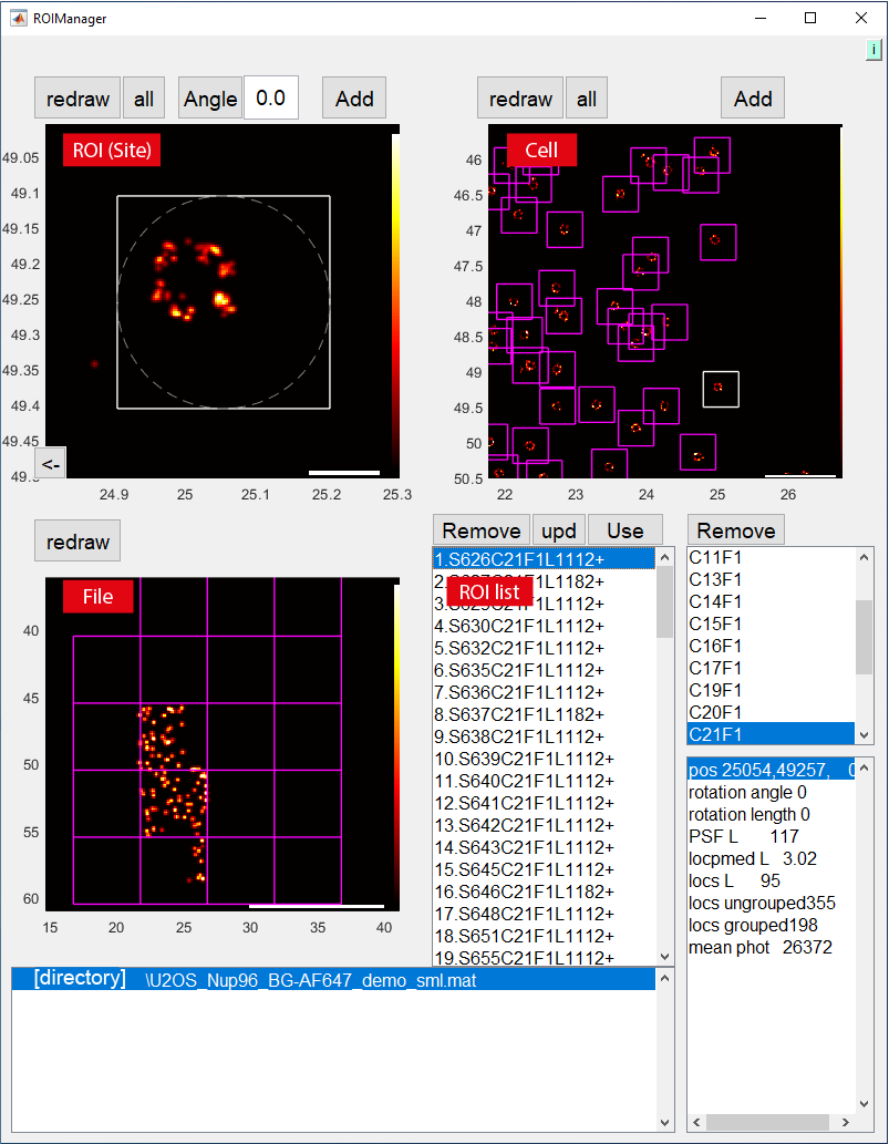
2. Now you see empty boxes. To show images properly, click the redraw button and one site as in the image above. The window should look like this now:

   

3. Click a few sites in the ROI list to display them.

Loading LocMoFit

Let us now start to work with LocMoFit by loading it into SMAP:

1. Go to the [ROIs] tab.

2. Go to [Evaluate] tab and click add module.

   

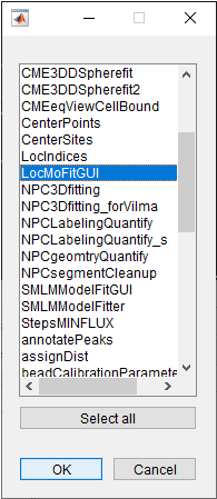
3. In the popup window, select LocMoFitGUI and click ok.

4. Show the LocMoFitGUI GUI by clicking on it in the list of loaded modules. Your SMAP window should look like this now:

   

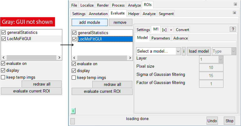
Note

The button in the up-right corner of the LocMoFit GUI provides details of fields/buttons in the current tab/sub-tab.

Setup

We will be using the model ring2D here (more about model types).

1. First, we have to load the model into LocMoFit:

   • In the right panel, go to [M1] -> [Model], click the drop-down menu (where select the model… is shown), and then select ring2D.

     

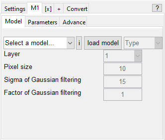
   • Click load model. Now the model is loaded.

   Note

   M1 stands for model 1. Find out more about the M1 tab here. LocMoFit allows you to load multiple models and combine them into a single composite model, which you will learn in the next tutorial.

   Note

   Clicking the button next to the drop-down menu opens the webpage detailing the selected model.

2. Next, we set up the parameter settings:

   • Go to the tab [Parameters]

     

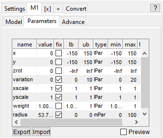
   • Fill in the table as followed (non-default values are in bold):

   name	value	fix	lb	ub	type	min	max
   x	0	☐	-150	150	lPar	-150	150
   y	0	☐	-150	150	lPar	-150	150
   zrot	0	☑	-Inf	Inf	lPar	-Inf	Inf
   variation	10	☑	0	10	lPar	0	20
   xscale	1	☑	1	1	lPar	1	1
   yscale	1	☑	1	1	lPar	1	1
   weight	1	☑	1e-05	1	lPar	1e-05	1
   radius	53.7	☑	0	0	mPar	0	100

   Important

   What do all these different elements mean? Let’s start with the fields name and type. name shows parameter names. type indicates the types of parameters:

   • lPar: extrinsic parameters, which are independent of the geometries. These parameters therefore apply to different geometries.

   • mPar: intrinsic parameters, which determine the shape of the geometry and therefore are geometry-specific.

   Parameters x and y are the xy coordinates of the model with respect to the center of the ROI. zrot is the rotation around the z-axis. xscale and yscale are the scaling of the model along the respective axes. variation is the extra variation, the uncertainties that cannot be solely explained by the localization precision. It basically defines how blurred the model is. The field fix indicates whether each parameter is fixed to a specific value or not. If checked, the corresponding parameter will not be estimated but fixed to the value defined in the field value.

   The field value defines the initial values of the parameters. The fields min and max define the search range of a parameter. We will discuss other fields later.

   With the settings, now you defined a ring with a radius = 53.7 nm. The ring can be moved in the xy plane freely from -150 to 150 nm.

Preview the model before fitting

In practice, you often have to optimize the fitting settings, especially finding good initial parameters. In this case, previewing the model with the initial parameters is useful.

1. To activate the preview mode, check the checkbox preview in the bottom-left corner of the tab [Parameters].

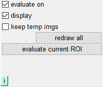
2. Go back to [Evaluate], make sure that evaluate on and display in the left panel are checked.

   Note

   • The loaded modules will be evaluated only when evaluate on is checked.

   • Result windows of the loaded modules will be displayed only when display is checked.

     

3. Now click on the first ROI in the ROI manager window and wait for a few seconds. You should see a new window LocMoFitGUI, in which the localizations are plotted on the initial model.

   

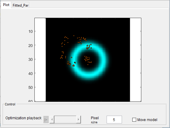
4. You can explore the data more by repeating these steps for a few more ROIs.

Fitting

Next, we will execute the fitting. This is done by clicking the site in the list of sites in the ROI manager window with the preview box unchecked:

1. Go back the tab [Parameters] and uncheck preview.

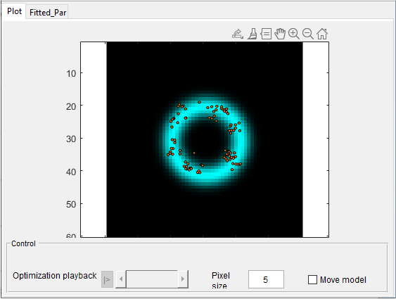
2. In the ROI list of ROI Manager window, click on site 1 and wait for a few seconds. You should see the updated LocMoFitGUI window displaying the fitted model.

   Note

   The LocMoFitGUI window allows you to inspect the result right after fitting. The window may look different depending on the model type.

Now you have your first fit done! Congratulations! You should see the previously uncentered structure now centered because the fit finds the position of the structure. You can further explore a few sites to get familiar with the interface.

Next tutorial

You are in the introductory series. The next tutorial is Composite model.